In a previous post, I described a method to detect a chord using a Fourier transform in Java/Scala. I’ve re-implemented the same in R, detailed below.
This will generate an audio file containing the C-Major chord:
library(sound)

c<-261.63
e<-164.81
g<-196

len<-1
cData<-Sine(c,len)
eData<-Sine(e,len)
gData<-Sine(g,len)

audio<-normalize(cData+eData+gData)

saveSample(audio, "out\\ceg.wav", overwrite=TRUE)
And a series of helper functions:
magnitude<-function(x) { sqrt(Re(x) * Re(x) + Im(x) * Im(x)) }
maxPitch<-audio$rate/2-1

frq<-c(16.35,17.32,18.35,19.45,20.60,21.83,23.12,24.50,25.96,27.50,29.14,30.87)
noteNames<-c("C", "C#0/Db0", "D0", "D#0/Eb0", "E0", "F0", "F#0/Gb0", "G0", "G#0/Ab0", "A0", "A#0/Bb0", "B0")

lookup<-data.frame(noteNames,frq)
A function to find the middle frequency in each FFT bucket:
idxFrq<-function(idx) { (idx - .5 ) }
And a function to find the closest note in the lowest octave:
noteDist<-function(note1, note2) { abs(log(note1)/log(2) - log(note2)/log(2)) %% 1 }
Now to do the actual FFT:
fftdata<-fft(audio$sound)
half<-fftdata[1:maxPitch]
indexes<-c(1:maxPitch)
magnitudes<-magnitude(half)
Now, from each bucket, find the note that is closest to each bucket:
closest<-function(x){ subset(lookup, select=c(noteNames,frq),subset=(min(noteDist(frq, x)) == noteDist(frq, x)))$noteNames }

noteList<-mapply(closest, indexes-0.5)
mag<-data.frame(noteList, magnitudes)
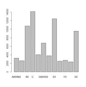
barplot(by(mag$magnitudes, mag$noteList, sum))
This results in the following image, which has peaks at C, E, and G, as expected.
The calculation is very crude – all frequencies are mapped to a note evenly, which isn’t really correct.
This can be adjusted by de-emphasizing the fft buckets between notes:
scale<-function(x){ .5 + .5 * sin(pi * x*2 + pi/2) }
note<-function(x) { 12 * log(x/440)/log(2) + 49 }
scaleData<-scale(note(idxFrq(indexes)))
scaledMagnitudes<-scaleData*magnitudes
scaledMag<-data.frame(noteList, scaledMagnitudes)
This looks better – the three highest are the notes in the chord-

