Got this from ChatGPT and tested.
Go to apps script:
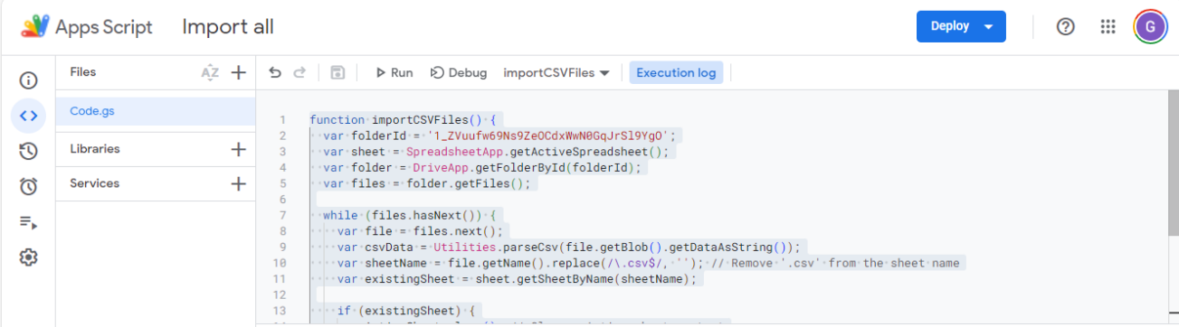
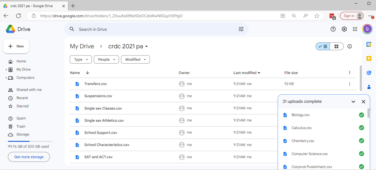
Paste the script below, add your folder ID, and save. The folder ID can be obtained from the URL to the folder:
Then, click Run – you will have to go through several security prompts to agree to trust the script.
function importCSVFiles() {
  var folderId = '1_ZVuufw69Ns9ZeOCdxWwN0GqJrSl9YgO';
  var sheet = SpreadsheetApp.getActiveSpreadsheet();
  var folder = DriveApp.getFolderById(folderId);
  var files = folder.getFiles();

  while (files.hasNext()) {
    var file = files.next();
    var csvData = Utilities.parseCsv(file.getBlob().getDataAsString());
    var sheetName = file.getName().replace(/\.csv$/, ''); // Remove '.csv' from the sheet name
    var existingSheet = sheet.getSheetByName(sheetName);

    if (existingSheet) {
      existingSheet.clear(); // Clear existing sheet content
    } else {
      sheet.insertSheet(sheetName); // Create a new sheet if it doesn't exist
    }

    var targetSheet = sheet.getSheetByName(sheetName);
    targetSheet.getRange(1, 1, csvData.length, csvData[0].length).setValues(csvData);
  }
}